SAMOVA 2.0

A program to define the genetic structure of populations by a simulated annealing approach

Introduction

Description of the algorithm

Input files

Output files

References

Download

Introduction

SAMOVA 2.0 implements an approach to define groups of populations that are geographically homogeneous and maximally differentiated from each other. As a by-product, it also leads to the identification of genetic barriers between these groups. The method is based on a simulated annealing procedure that aims at maximizing the proportion of total genetic variance due to differences between groups of populations (SAMOVA, Spatial Analysis of MOlecular VAriance). The method is described in Dupanloup, Schneider and Excoffier (2002).

A new functionality of SAMOVA 2.0 is to define groups of populations that are maximally differentiated from each other, without constraint for the geographic composition of the groups.

SAMOVA 2.0 runs on Windows. There is no Linux or Mac version yet.

Description of the algorithm

Groups of populations are geographically homogeneous and maximally differentiated from each other

Preliminary steps

A set of Voronoi polygons is constructed from the geographical location of the n sampled points.
An arbitrary partition of the n populations into K groups is initially chosen at random.
The genetic barrier(s) between the K groups are identified as edges of Voronoi polygons separating groups of populations.
The FCT index associated to the K groups is computed.

Simulated annealing steps

We select an edge at random on a given barrier.
The two populations located on both sides of the selected edge are identified, and one population chosen at random is assigned to the group of the other population.
The genetic barrier is modified by updating the list of edges separating the new groups of populations.
The new FCT value (noted FCT*) associated with the new partition is computed.
The new structure is accepted with probability

where S is the number of steps performed in the simulated annealing process, and A is an arbitrary constant controlling the speed of the cooling process.

In SAMOVA 1.0, the number of steps S in the simulated annealing process was set to 10 000 and the constant A to 0.9158. In this case, the probability p defined above is equal to 1% if the difference between FCT and FCT* at the 10 000th iteration is equal to 0.001. In SAMOVA 2.0, S and A can be chosen by the user. You'll find below different combinations of values of S and A and the corresponding probability values to accept the new structure

FCT-FCT*	S	A	p
-0.1	10000	0.915811421	1E-200
-0.01	10000	0.915811421	1E-20
-0.001	10000	0.915811421	0.01
-0.1	100	1.831622842	1E-200
-0.01	100	1.831622842	1E-20
-0.001	100	1.831622842	0.01
-0.1	1000	1.221081895	1E-200
-0.01	1000	1.221081895	1E-20
-0.001	1000	1.221081895	0.01
-0.1	100000	0.732649137	1E-200
-0.01	100000	0.732649137	1E-20
-0.001	100000	0.732649137	0.01
-0.1	1000000	0.610540947	1E-200
-0.01	1000000	0.610540947	1E-20
-0.001	1000000	0.610540947	0.01

To make sure that the final configuration of the K groups is not affected by a given initial configuration, the simulated annealing process is repeated 100 times, starting each time from a different initial partition of the n samples into the K groups. The configuration with the largest associated FCT value after the 100 independent simulated annealing processes is retained as the best grouping of populations.

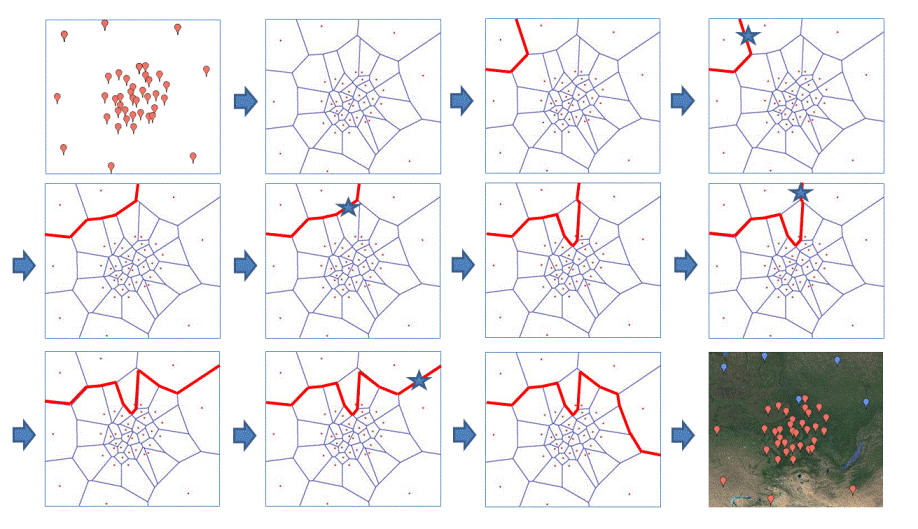
The cartoon below illustrates the behaviour of SAMOVA 2.0.

simulated annealing steps for geographically homogeneous groups

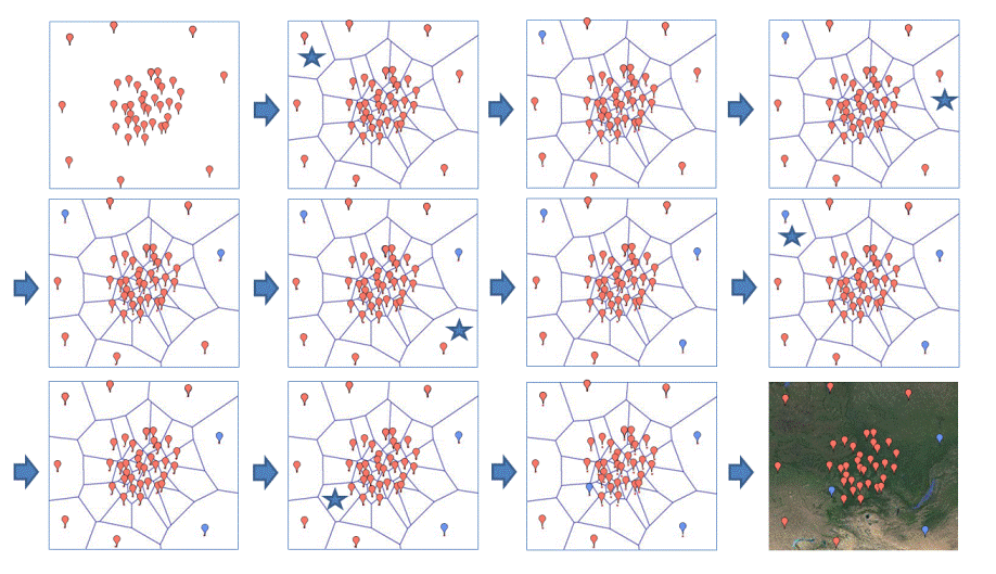
The cartoon below illustrates one case encountered frequently with SAMOVA 2.0: the allocation of one population from one group to another leads to the fragmentation of one group in 2 distinct sets of adjacent populations.

simulated annealing steps for geographically homogeneous groups leading to discontinuous

Groups of populations are maximally differentiated from each other, without constraint for the geographic composition of the groups

Preliminary steps

An arbitrary partition of the n populations into K groups is initially chosen at random.
The FCT index associated to the K groups is computed.

Simulated annealing steps

We select a population at random
We assigned this population to another group, chosen at random.
The new FCT value (noted FCT*) associated with the new partition is computed.
The new structure is accepted with probability

where S is the number of steps performed in the simulated annealing process, and A is an arbitrary constant controlling the speed of the cooling process.

The cartoon below illustrates the behaviour of SAMOVA 2.0.

simulated annealing steps without constraint for the geographic composition of the groups

Input files

There are 2 ways to run SAMOVA 2.0 :

using the command line: samova2_console.exe INPUTFILE.SAR. In this case, INPUTFILE.SAR should contain all the parameters SAMOVA 2.0 needs to run.
double clicking on samova2_console.exe. In this case, SAMOVA 2.0 will ask you the name of your input files and to specify the parameters for the run

SAMOVA 2.0 (like SAMOVA 1.0) needs two input files. The first one (*.geo) must contain the geographic coordinates of the sampling localities of your populations. The second one (*.arp) is an Arlequin input file containing the genetic data sampled in your populations. The Arlequin file must have the SAME NAME as the geographical file with the extension (*.arp). The order of the populations in the two input files MUST BE THE SAME !!!

The file containing the geographic coordinates of the sampling localities of your populations must have the .geo extension.
Important notice: SAMOVA 2.0 does not work if two sampling localities have the same geographical coordinates.
The geographical input file must be structured the following way. Each line corresponds to a population. Each line must contain five fields separated by TAB characters:

an integer number corresponding to the line in the file
the name of your population within quotes
the longitude of your sampling point
the latitude of your sampling point
an integer (for example, 1).

Examples of input files are given below:

When SAMOVA 2.0 runs, it expects the generic name of your input files. If you have INPUTFILE.GEO and INPUTFILE.ARP as input files, it will expect to read INPUTFILE (either in the INPUTFILE.SAR file or from the standard input).

Output files

A set of output files are created by SAMOVA:

SAMOVA2.log: this file contains all the steps done by SAMOVA 2.0 and, in case of problems, the location of the problems
SAMOVA2_short.log: this file contains the final composition of the groups of populations
SAMOVA2_finaltruct_geo.arp: an arlequin project file created by appending the input arlequin project file with the genetic structure defined by SAMOVA 2.0 (groups are geographically homogeneous)
SAMOVA2_finaltruct_geo.res: a directory with the results of an AMOVA performed by Arlecore 3.5 on SAMOVA2_finaltruct_geo.arp
SAMOVA2_results_geo.htm: this file contains a map of the sampling points with different groups of populations defined by SAMOVA 2.0 (groups are geographically homogeneous)
SAMOVA2_finaltruct_nogeo.arp: an arlequin project file created by appending the input arlequin project file with the genetic structure defined by SAMOVA 2.0 (without constraint for the geographic composition of the groups)
SAMOVA2_finaltruct_nogeo.res: a directory with the results of an AMOVA performed by Arlecore 3.5 on SAMOVA2_finaltruct_nogeo.arp
SAMOVA2_results_nogeo.htm: this file contains a map of the sampling points and the groups of populations defined by SAMOVA 2.0 (without constraint for the geographic composition of the groups)

References

Dupanloup, I., Schneider, S., Excoffier, L. (2002) A simulated annealing approach to define the genetic structure of populations. Molecular Ecology 11(12):2571-81.