SIMCOAL2

A coalescent program for the simulation of complex recombination patterns over large genomic regions under various demographic models

Introduction

We present here SIMCOAL2, an extended version of the SIMCOAL program (Excoffier et al. 2000), to simulate the neutral genetic diversity at partially linked loci under different histories and a wide range of migration and demographic models.

SIMCOAL2 includes a number of new features compared to the previous version:

1. The possibility of arbitrary recombination rates between adjacent loci

2. Multiple coalescent events per generation, allowing the correct simulation of very large samples and very large recombining genomic regions

3. The simulation of SNP data with arbitrary minimum frequency, for instance to simulate ascertainment bias

4. The output of diploid genotypic data generated under the assumption of Hardy-Weinberg equilibrium

5. The simulation of a mixture of different data types (DNA sequence, RFLP, STR, or SNP) along a single chromosome.

Recombination

A recombination event can be schematically represented as follow: 

Schematic representation of a recombination event backward in time

Assuming that at a given generation t we sampled 4 partially linked genes (loci) arbitrarily distributed on a given chromosome segment C. A recombination event (represented byon the drawing) creates two new lineages in the ancestral generation, t+1, here arbitrarily called A₁ and A₂. A₁ receives from C a copy of the genes located to the left of the recombination event, while A₂ receives a copy of the genes located on the right side of the recombination event. The copies of the genes shown in black are not observed in the present sample and thus have an unknown origin. We make this distinction between known (white) and unknown (black) genes, because we only have to simulate the ancestry of the observed genes. Therefore, we are only interested in the recombination events occurring between white genes. The other recombination events (e.g. between the first two genes in A₂) have no effect on the genetic constitution of the sample, and thus do not need to be followed or simulated. The simulation of the coalescent process with recombination is stopped when the Most Recent Common Ancestor (MRCA) of each locus is found.

The recombination rate is allowed to vary between adjacent loci in order to simulate arbitrary patterns of recombinations along a chromosome, e.g. the occurrence of recombination hot-spots. The following Figure gives an example of a simulated recombination pattern. Here, four haplotypes blocks (noted as B1 to B4) characterized by low recombination rate are interrupted by three hotspots of recombination (HS1 to HS3). The height of the bars are here proportional to the recombination rates between adjacent loci.

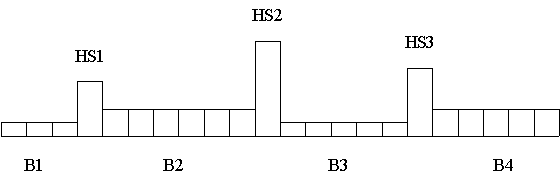
Representation of relative recombination rates across a chromosomal segment

Validation of the simulations: The expectation of the number of recombination events in the genealogy of two chromosomes studied for two partially linked markers was used to check the accuracy of our simulations. For two markers separated by the recombination fraction r,  the expected number of recombination events having occurred since their Most Recent Common Ancestor is equal to 6R/(R+6), where R=4Nr (eq. 31 in Simonsen and Churchill 1997) and N is the population size. We report below the comparison between theoretical predictions and the average values obtained from  the simulation of 10 000 genealogies with SIMCOAL2.

Multiple coalescent events

The time to the MRCA (T_MRCA) at any locus (measured in units of M generations, where M=N for a haploid population, and M=2N for a diploid population) is independent from the recombination rate. Under the standard coalescent model where only one coalescence per generation is assumed, the expected T_MRCA is given by 2(1-1/n), where n is the number of sampled gene copies. When the sample size is not small with respect to the effective size (Wakeley 2003), or when the recombination rate is high leading to the progressive generation of a large number of ancestral chromosome segments (and thus increasing the number of gene lineages in past generations), multiple coalescent events needs to be implemented to avoid an overestimation of the T_MRCA at any locus. Because this procedure is computationally intensive, we only implement it if the effective number of gene lineages in a deme (at any given time in the past)  is large compared to the local deme size N. On the Figure below, we present the average T_MRCA obtained over 10 000 simulations of 100 uniformly distributed SNPs with initial sample size n=100, and an overall recombination rate of 4NR=100. The mean and standard deviation between loci are equal to 1.98 and 0.01 respectively. The straight line gives the theoretical prediction under the standard coalescent model (T_MRCA = 1.98).

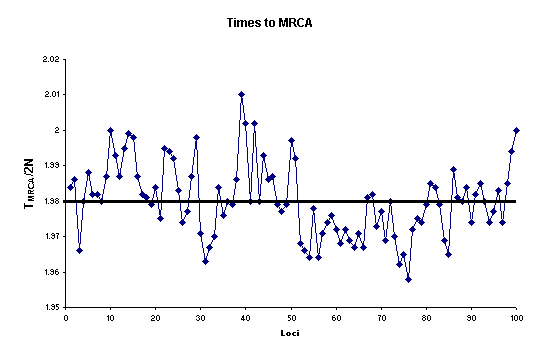
Distribution of T_MRCA at 100 adjacent partially linked loci

SNP data

With SIMCOAL ver 2.X users can generate the same data types as with  SIMCOAL ver 1.0 (RFLP, DNA sequence, and microsatellite data), plus Single Nucleotide Polymorphims (SNP) data. We also offer the possibility to simulate SNP with a minimum frequency for the minor allele (which can be different for every SNP) in order to mimic one form of ascertainment bias. A SNP locus is modeled as a DNA base pair where one mutation has appeared somewhere at random along the genealogy of the locus. As shown in the following figure, the location of the mutation on the tree determines its frequency in the sample.

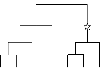
Schematic representation of a SNP-defining mutation on a gene genalogy

Several chromosome structures

With the new release of SIMCOAL ver 2.1, it is now possible to simulate a much more flexible chromosomal structure than before. We now indeed offer the possibility to simulate the evolution of several chromosomes. By chromosomes we mean independent chromosomal segments. Users can simulate one or more (no limitation except hardware) chromosomes each one exhibiting its own number of blocks, its own number of markers, its own kind of markers etc... The input files used with SIMCOAL2.1 are thus different from those of  SIMCOAL2.0 released earlier this year. The portions used to set up the populations features and their history are unchanged and the only differences are about the definition of the chromosomal segments. An example of a new input file is given below.

Generalized Stepwise mutation model << NEW >>

In SIMCOAL ver 2.1, we introduce a more realistic mutation model for STR markers: the Generalized Stepwise Mutation (GSM) model, which allows insertion (deletion) of more than one repeats. The number of repeats inserted (deleted) in one mutation event is treated as a random variable, and is randomly drawn from a Geometric distribution with parameter p. The value of p can be given in the input file (see below). The expectation and variance of the Geometric distribution are E[s]=p/(1-p) and Var[s]=p/(1-p)², respectively, where s+1 is the number of mutational steps. Concretely this means that for a parameter p set up to 0 in the input file, the number of repeats inserted (deleted) will be equal to one for every mutation event. When p is set up to 0.5 in the input file, the expected number of repeats inserted (deleted) is equal to 2 with a variation around the mean is given in the following scheme.

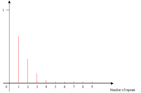
Distribution of the number of repeats inserted (deleted) according to a geometric law with parameter p=0.5

Input files

A single input file is needed for the simulation. The format of the input file is differs from the format used in SIMCOAL ver 1.0. The parameters required are listed bellow. The differences between the two versions of SIMCOAL are indicated using different colors. We show in blue the unmodified parameters, and in red the modified and new parameters.

Example of an input file

Definition of the history of population: Suppose that we want to simulate a scenario of a population trifurcation, where a (haploid) founder population of size N= 2 000 (note that it would be equivalent to the simulation of a diploid population of size N=1000) splits into 3 daughter populations of size 1,000, 2,000 and 1,000, respectively,  where 20, 30 and 10 genes are respectively sampled. After the fission event, we shall assume that the three daughter populations are not completely isolated and can exchange genes at rate m=0.005 per generation, which is also assumed constant over time. 

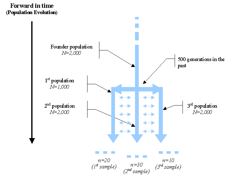
Schematic representation (viewed forward in time) of a population trifurcation

While the history of the populations is naturally described forward in time (black arrow on the left above),  users simulating a coalescent process have to think backward in time as in the following  Figure.

Schematic representation of the backward historical process actually simulated by SIMCOAL

The specification of the process to be simulated proceeds as follows:

1. Starting at the current generation (0) with three samples of size of 20, 30 and 10 genes, SIMCOAL simulates generation after generation the demography of the populations and the coalescent process backward in time. We first start by defining how many demes we need to simulate, as well as their size, and the number of samples genes:

//Input parameters for the coalescence and recombination simulation program : simcoal2.exe
3 samples to simulate
/Deme sizes (haploid number of genes)
1000
2000
1000
//Sample sizes
20
30
10
 

2. If users have defined migration (as it was the case in the example), they have to specify the total number of migration matrices that will be used during the simulation, as well as which migration matrix (see here to have more details) is to be used at any time. Unless specified otherwise (by an historical event) SIMCOAL uses the migration matrix having  id number equal to 0 at the begining of the simulations (generation zero). This migration matrix will be then used until users specify another matrix to be used with another historical event. In our case we just need to define two migration matrices. The second one has only zeroes, implying that the demes will not exchange migrants anymore. Note that diagonal elements are here set to zero, but these values are not used by SIMCOAL.

//Number of migration matrices : If 0 : No migration between demes
2
//Migration rates matrix 0 : 
0.000 0.005 0.000
0.005 0.000 0.005
0.000 0.005 0.000
//Migration rates matrix 1 : No migrations
0 0 0
0 0 0
0 0 0
 

3. In our example, migrations are allowed for the first 500 generations and are disallowed after the fusion of the three demes into one (when looking backwards). The population fusion and the change of migration matrix are specified by just two historical events:

//Historical event: time, source, sink, proportion of migrants, new deme size, new growth rate, new migration matrix
2 historical events
500 0 1 1 1 0 1
500 2 1 1 1 0 1

The first parameter (shown in red) represents the time at which occurs the historical event (in number of generations in the past relative to present time). The last parameter (shown in red as well) is the id of the new migration matrix. Thus, the first historical event states that: 500 generations ago, deme #0 (first population defined in the input file) will send all its genes to deme #1, and deme zero will remain at the same time as before, but a new migration matrix (#1) should be used from now on. the second historical event specifies that deme #2 should send all its genes to deme #1, and that migration matrix #1 should be used afterwards. Therefore at generation 501, all remaining gene lineages should be present in deme #1, and since no migrations are allowed, they will remain there until they all coalesce and the simulation stops.

Definition of the genetic structure of chromosomes: Suppose that we want to simulate the genetic diversity expected of a chromosomal segment  made up of three blocks of partially linked loci (recall that by block we mean a set of identical genetic markers with the same inter-locus recombination rate), each one being separated by a recombination hot-spot, as shown in the following Figure. Assume that the first block contains 25 SNPs, that the second block contains 50 microsatellite (STR) loci, and that the last block is also made up of 25 SNPs.

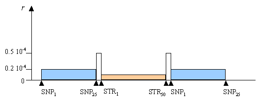
Recombination distribution to be simulated

If the blocks were each of consisting of 155 Kb, an assuming a diploid size of N=10,000, the recombination rate between adjacent loci (r) within the 3 blocks would be equal to 0.2 x 10^-4, 0.1 x 10^-4 and 0.2 x 10^-4 , respectively. We shall finally assume that these blocks are separated by two recombination hot-spots of with recombinations rates  r = 0.5 x 10^-4. 

Therefore, users will first have to set up the number of simulated blocks that they want to simulate. Here, this number is 5 because we need to include the two recombinations hot-spots. In SIMCOAL2, a block is defined as a set of adjacent markers with the same features and the same recombination rate between adjacent markers.  A block can therefore be viewed as a chain of b elements. Every element has two attributes, which are the specificities of the genetic marker (see here to have more details on how to specificify the properties of the markers like its type, its mutation rate, etc... ) and the recombination rate with the next element. In the following scheme, the length of the links between markers is proportional to the recombination rate. 

 Note that the link between blocks i and i+1 will therefore depend on the recombination rate on the right of the last marker of block i. We therefore need to define a transition block (block2 in the previous scheme) made up of a single SNP with a large recombination rate in order to simulate the recombination hot-spot between the SNP#25 and  the STR#1. In the input file these 3 blocks are defined as follows

With these three blocks, we can simulates 25 SNPs with adjacent recombination rates equal to 0.00002, separated from 49 STR (with adjacent recombination rates equal to 0.00001  by a hot spot of recombination (recombination rates between SNP#25 and STR#1  equal to 0.00005). An identical structure would need to be described to simulate the second recombination hot-spot after the STR#50). Note that the last element of the last block is a special element, since its recombination rate is irrelevant, and ignored by SIMCOAL

With this kind of specifications, users are free to simulate any chromosomal structure they want, concerning the intensity of recombination rates but also the types of markers and the mutation rates.

For instance, if one would like to simulate 4 STRs with different mutation rates,  with arbitrary recombination rates ( i.e. arbitrarily spaced on a chromosome), users would need to define 4 blocks of 1 STR as

The following listing shows how to set up the complete input file to perform the  simulations a trifurcating population described above.

Summary of the different parameters needing to be defined for the description of the markers to be simulated

The parameters which can be given for every markers are: 
MICROSAT [number of loci] [recombination rate] [mutation rate] [Geometric parameter << NEW >>] [range constraint]
SNP              [number of loci] [recombination rate] [minimum frequency]
DNA             [number of loci] [recombination rate] [mutation rate] [transition rate]
RFLP            [number of loci] [recombination rate] [mutation rate] 

[number of loci]                   :  Number of partially linked loci in a block 
[recombination rate]            :   recombination rate between adjacent markers in a block   (Global recombination rate of the block = [recombination rate] *([number of loci]   -1))
[mutation rate]                    :   mutation rate for every marker in a block                           (Global mutation rate of the block          = [mutation rate] *[number of loci])
[Geometric parameter]        :  parameter for the Geometric distribution (varies between 0 and 1)
[range constraint]                :  0 or 1 means no constraints, higher numbers give the maximum number of repeats
[minimum frequency]           :  minimum frequency of a SNP in the whole set of population (ascertainment bias) 
[transition rate]                    :  fraction of substitutions that are transitions

Additional examples of input files for SIMCOAL (without recombination) can be found on this page .

Output files

The final state of each gene is recorded and output to several files according to two data formats. The first format is compatible with the Arlequin program (Schneider et al. 2000). The data generated after each simulation are output to a separate Arlequin project file. An Arlequin batch file is also created, listing all simulated files, and allowing one to compute different statistics on the whole set of simulated files with Arlequin. it therefore allows one to obtain their distribution after extraction from the Arlequin output files. Note that with version 2.0 of Arlequin, a utility is provided to collect most statistics computed in the analysis of batch files under the form of MS-Excel compatible files. Examples of statistics that can be extracted from batch file analysis by Arlequin are: nucleotide composition, gene diversity, homozygosity, mean number of pairwise differences, number of haplotypes, number of polymorphic sites, Tajima’s D, Fu's F_S, extent of linkage disequilibrium among loci, mutation parameter q = 2Nu estimated from homozygosity, mean number of pairwise differences, number of polymorphic sites, or number of alleles, and genetic distances based on pairwise F_ST’s. Note also that the Arlequin software has a file conversion utility for exporting input data files into several other format like Biosys, Phylip, or GenePop, so that files produced by SIMCOAL2 could be also analyzed by these software's after file conversion.

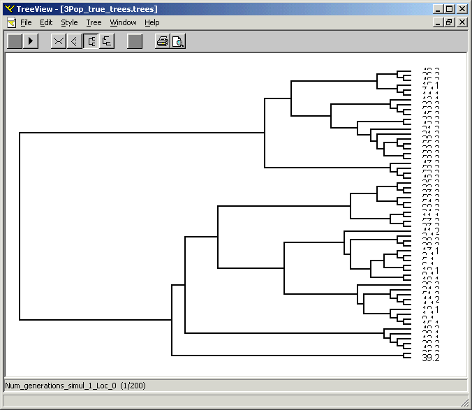
The two other sets of output file produced by SIMCOAL2 are compatible with the NEXUS file format. Two files with the “*.trees” extension list all the genealogical trees for each simulated locus. The branch lengths are expressed either 1) in units of generations scaled by the population size (N), and therefore representing the true coalescent history of the sample of genes, or 2) in units of average number of substitutions per site (except for data sets containing SNP markers), and therefore representing the realized mutational tree. These two sets of trees can be visualized with the software TREEVIEW (Page 1996), as shown on the figure below. Finally, a file with the “*.paup” extension, lists all the simulated genes together with their true genealogical structure. This file can be analyzed with David Swofford's PAUP* software (1999). Because, these files can be huge, we do not produce them by default, and a conditional compilation directives (#define _PRINT_TREE_PAUP_ and ) must be uncommented in the source code of "cond_var.h", and the source must be recompiled to reflect these changes.

Unlike SIMCOAL ver 1, SIMCOAL ver 2 stores all the output files in a folder automatically created and named according to the name of the input parameter file (without the extension .par). Beware, SIMCOAL2 does not clean your disk. For example: if you run a first set of 1000 simulations and a second set of 100 simulations using the same input parameter file, only the first 100 Arlequin (*.arp)  files will be updated. The others will be kept on your disk without any changes.

Computation times

The speed of simulation with recombination can be much slower than without recombination, and will increase with sample size, effective population size, the number of loci, and the total recombination rate. For instance, SIMCOAL2 needs 15 minutes to simulate 10,000 samples of 100 diploid individuals (n=200 and N=1,000) typed at 250 SNPs over a segment of 250 Kb (assuming 1cM = 1Mb, and thus with total recombination rate R=4Nr=10 for the whole chromosome segment), and about 2.5 hours to simulate 10,000 samples of 250 microsatellite loci over 2.5 Mb (total recombination rate R=100), using a Pentium 4 (2.8Ghz) under the Linux operating system.

Installing and running SIMCOAL2

The archive of executable files for windows and Linux includes the compiled files simcoal2.exe as well as examples of input files to simulate partially linked SNPs,  microsatellites and a mixture of these data types. After extraction, there are three ways to run simcoal:

1. simcoal <no arguments>
   The program will prompt you for :
   a) an input file name to process (just enter the name of the file without the ".par" extension )
   b) the number of simulations to perform.  
   c) a boolean flag to indicate if you want to generate haplotypic (0)  or genotypic (1) data.
   
   
2. simcoal <batch file name>
   The program will open the batch file that should contain, on the first line, the number of simulations to perform, and on the following lines the names of the input files to process
   Example: simcoal testbatch.txt
   
   
3. sim_coal <file name> <number of simulations to perform> <haplotypes (0)/ genotypes (1)>
   Example: simcoal MIX.par 1000 0
   

The source files can be compiled with Borland C++ Builder v. 5 and v. 6 to run SIMCOAL2 on windows (2000/XP), or with gcc (GNU project) to run SIMCOAL2 on a Linux Operating System. To compile the source code under Linux, uncomment the line "#define _LINUX_" in the file "cond_var.h". Others compilation options are also listed in the file "cond_var.h", and enable SIMCOAL2 to produce additional (undocumented) output files, mainly used for debugging purposes.

References

• Page RD, 1996. TREEVIEW: An application to display phylogenetic trees on personal computers. Comput. Appl. Biosci. 12(4):357-358.

• Schneider S, Roessli D and Excoffier L, 2000. Arlequin: a software for population genetics data analysis. User manual ver 2.000. Ver. 2.000. Geneva: Genetics and Biometry Lab, Dept. of Anthropology, University of Geneva.
  http://lgb.unige.ch/arlequin

• Simonsen KL, and Churchill GA, 1997. A Markov chain model of coalescence with recombination. Theor. Popul. Biol. 52(1): 43-59.

• Wakeley J, and Takahashi T, 2003. Gene genealogies when the sample size exceeds the effective size of the population. Mol. Biol. Evol. 20(2):208-213.

Versions

•  SIMCOAL  :  Simulate coalescence in populations with complex history (migrations, demographic fluctuations, etc...)  download it.

•  SIMCOAL2  :  Extension of SIMCOAL. Simulate coalescence + recombination (uniform recombination rates, hot spot etc...), all kind of coalescent events (when sample sizes are small), a new kind of marker (SNPs) and a mixture of different markers. 

•  SIMCOAL2.1  :  Extension of SIMCOAL2. Simulate several chromosomes with different structure, Generalized Stepwize Mutation model for microsatellites. 
  •  SIMCOAL2.1.1  : correction of a bug concerning the Stepwize Mutation Model with range constraint 
  •  SIMCOAL2.1.2  : correction of a bug concerning simulations with sample sizes equal to 0.  latest release (download on the top). Now simcoal2 accepts to simulate empty populations (population with sample sizes equal to 0), provided that there is at least one population with sample size higher than 0.

Bug report

• 22 03 2005: A bug was introduced in the version 2.1 concerning the range constraint option for microsatellites when there is no recombination - Corrected in the latest release SIMCOAL2.1.1
• 14 09 2005: A bug concerning simulations with sample sizes equal to 0 was corrected in the latest release SIMCOAL2.1.2 (download on the top).

Guillaume Laval, Computational and Molecular Population Genetics Lab, University of Bern

Last edited on 14.09.05 (16:14)